On-line version of a contribution to the
Third GLOREAM
Workshop, Ischia, Italy, September 1999.
If you have problems to view the math included in this paper, please follow
these instructions.
Inverse modelling of the ETEX-1 release with a Lagrangian particle
model
Petra Seibert1
Institute of Meteorology and Physics
University of Agricultural Sciences
Türkenschanzstr. 18, A-1180 Vienna, Austria
seibert_+aT+_.ac.at,
http://www.boku.ac.at/imp/envmet/
Andreas Stohl
Lehrstuhl für Bioklimatologie und Immissionsforschung,
Technical University of Munich, Freising, Germany
http://www.fw.tum.de/LST/METEOR/stohl/astohl.html
Abstract
| The derivation of source-receptor matrices for a passive, nonreacting
and nondepositing tracer from backward runs of a Lagrangian particle
dispersion model is shown. This technique is applied to the first
release of the European Tracer Experiment ETEX. The source-receptor
matrix is used to invert measurements to obtain the temporal evolution
of the release with given release location as a first illustration and
test of the method. |
1 Introduction
The purpose of this study was to test the potential of inverse
modelling with data from the European Tracer Experiment ETEX
[2,]. In this context, inverse modelling means to
derive information on a source of an atmospheric trace constituent from
ambient concentration measurements, using a dispersion model for the
description of the source-receptor relationship. At first, we show how
a Lagrangian particle dispersion model (LPDM) can be used in a backward
mode to derive source-receptor matrices. This is a novel approach. Then
the technique is applied to the ETEX release and a regularised
inversion is performed to deduct the temporal evolution of the
release. This is, however, just a very first application, and the
outlook outlines possible refinements and further evaluations.
There are a number of different approaches to inverse modelling of
atmospheric trace constituents. For a linear problem (ambient
concentrations proportional to the source strength), one can obtain the
unknown source from the solution of a linear system of equations, with
measurements as knowns and elements of the source-receptor matrix (SRM)
as coefficients. Depending on the number of knowns and unknowns as well
as the conditioning of the matrix, one often needs to apply a so-called
regularisation (input of a-priori knowledge) [6]. The SRM can
be obtained by forward or backward modelling, and with a Lagrangian or
a Eulerian model. The backward approach is most efficient when the
number of unknown source elements exceeds the number of measurements.
Lagrangian models have the advantage compared to Eulerian models that
they have a better numerical accuracy (mainly, no numerical diffusion
due to the advection scheme), and that they do not suffer from a grid
resolution problem near point sources. In the backward mode, this is
especially important because measurements are almost always made at a
point or along a line (aircraft) and with Eulerian models one would
need to apply a near-source sub-model or else loose once more in
accuracy.
The other approach is to search iteratively for the minimum of a cost
function, made up by the misfit between measurements and model, and a
regularisation term if necessary. This requires the calculation of the
gradient of this cost function with respect to the source elements.
Often, this approach is realised with a Eulerian model and its adjoint,
the only viable approach for large nonlinear problems [1]. It
is also possible to use a Eulerian model and its adjoint for the
determination of a SRM by defining suitable cost functions.
2 Derivation of the source-receptor matrix
2.1 Forward and backward simulations with a LPDM
In the forward mode, particles are released from prescribed source
areas, and transported with the mean and turbulent velocity field. They
carry a mass depending on source strength and particle release rate.
It can be altered by processes such as deposition or decay.
Concentrations are calculated by summing up the masses of all the
particles in a grid cell, and dividing the sum by the cell's volume.
In the backward mode, used for inverse modelling, the same formalism and
computer model are applied, but the particle trajectories are
integrated backward in time, using a negative time step. However,
there is a new interpretation: particle masses are replaced by mixing
ratios c º c/r (where c is the mass concentration and
r the air density) in an infinitesimal volume of air. In our
Lagrangian frame of reference, c can change only by sinks such as
deposition or decay and by uptake of emissions. Without deposition, the
individual rate of change of the mixing ratio is
where Sc denotes the alteration of c by sources S+ and sinks
S-.
The sources are independent of c, and sinks not considered as we
are dealing with an inert tracer2. Eq. 1 can be
easily integrated, yielding the instantaneous concentration. In ETEX
(and many other practical applications), measured concentrations
represent a point in space and an average in time (ETEX: sampling
interval 3 h). Thus, we need to average in time. If this averaging
time exceeds substantially the time scale of the turbulent
fluctuations, the temporal averaging alone is sufficient and additional
ensemble averaging is not necessary. Next, we introduce a
discretisation in time (index j) with J back trajectories in equal
intervals between t1 and t2, and index i for the temporal and
spatial variation of S+ (``gridded in space and time''):
|
|
c
|
º |
1
t2-t1
|
|
ó
õ
|
t2
t1
|
c(x,t)dt » |
å
i
|
|
é
ê
ë
|
S+i ( |
1
J
|
|
å
j
|
Dt¢ij) |
ù
ú
û
|
. |
| (2) |
The term in parenthesis on the right-hand side is equal to
Dti, the average residence time of all J trajectories
in a spatio-temporal cell i contributing to the measurement under
consideration.
Let us now consider that we have not just one
measurement, but many (different sites and times), denoted by l.
Then we see that the elements of the desired source-receptor matrix
M are
If we call the vectors of observations ([`(c)]l) and
emissions (S+i) y and x, respectively, we arrive at
the linear system of equations (LSE) to be solved for the inverse
modelling:
If the density variations between the receptors and the sources are
small, mixing ratios c may be substituted by mass concentrations,
and S+ by the emitted mass per volume and time, the parameter used
normally. Otherwise, c and S+ can be transformed with the air
density (climatological values are sufficient).
2.2 Implementation in the Lagrangian particle model FLEXPART
The Lagrangian particle dispersion model FLEXPART (details see
section 3.2) was used in this application.
FLEXPART gives gridded concentration fields as output. How can we
obtain gridded residence times from this output?
The time-averaged concentration in a grid cell [`c]i
as computed in FLEXPART can be written as
|
|
_
c
|
i
|
= |
mtot
Vi NJ
|
|
N
å
n = 1
|
|
J
å
j = 1
|
fijn, |
| (5) |
where Vi is volume of the grid cell,
N the number of instants in time used to form a temporal average
over an interval DT, mtot the total released mass, and
fijn the fraction of the mass of a particle attributed to a
specific grid cell, considering that all J particles have the same mass
because there are no sinks.
Using the residence fraction f, the average residence time
Dti during DT can be calculated as
|
Dti = |
DT
NJ
|
|
N
å
n = 1
|
|
J
å
j = 1
|
fijn. |
| (6) |
Combining (5) and (6), we obtain
This means that the desired residence times can be obtained by a
backward run of the regular FLEXPART model, transforming
the resultant concentrations according to (7). The spatial and
temporal resolution of the sources is given by the Vi and DT
used in the concentration calculation of FLEXPART.
3 ETEX application
3.1 Key features
The European Tracer Experiment ETEX
comprised two releases of a gaseous,
nondepositing, inert tracer. We are dealing here only with the first
one. This experiment can be characterised as follows [2,]:
- Release location: Bretagne (NW France)
- Release time: 23 Oct 16:00 UTC - 24 Oct 3:50 UTC, 1994 (11:50 h duration)
- Release rate: 7.98 g/s (constant)
- Sampling network: 168 stations over most of western and central Europe
- Sampling resolution: 3 hours
- Sampling duration: 30 intervals (90 h)
In the context of backward modelling, confusion can easily arise
because, for example, the physical receptors are used as sources in the
inverse model runs, whereas the physical source location acts as a
receptor location. Therefore, we introduce the following notation:
Source, concentration, receptor, etc. denote the
physical system or a forward simulation; the same words with a * refer
to the backward simulation. Thus, for example, a receptor is used
as a source*.
3.2 FLEXPART setup for the inverse model run
FLEXPART
is a LPDM developed by Andreas Stohl, and
tested on various tracer experiments [8]. It performed well for the ETEX-1
release (correlation coefficient between observations and simulated
concentrations 0.59, fractional bias 0.01).
FLEXPART was run with the following specifications:
- Input: ECMWF fields (1.0°, 31 levels as spatial and 3 h
as temporal resolution).
- 30 backward runs (one for each sampling interval)
- 10,000 particles released from each monitoring site
- each monitoring site (release* location) is one species
- output sampled with 3 h intervals on a 41×21 grid
with 1° resolution, 9 vertical cells
(0/75/150/300/600/1200/2400/3600/4800/6000 m), 35 time intervals
Thus, the size of our source-receptor matrix is
(41×21×9×35) × (168×30) = 180,810
× 5,740 » 1.4 ·109 elements. In sparse matrix
format, this amounts to » 300 MByte of data. This matrix is too
big for direct evaluation. Therefore, we have to consider the following
options for simplifications:
1) Take only the lowest layer (or a vertical integral) as potential
source, as concentrations* were well mixed near the release site.
2) Assume either the location as given (sample application: nuclear
power plant accident), or release time (sample application: nuclear
explosion with explosion time known from nuclide ratios).
3) Start with a coarse source resolution and narrow
it down iteratively while reducing the domain size, horizontally,
vertically, and/or temporally.
Here, we have applied simplifications 1 and 2 (release location given).
3.3 First visualisation of results
For a first visualisation, we plot fields that would result if a
backward simulation would have been made with releases* proportional to
the measured concentrations at each receptor. The plot may show
horizontal fields for one time interval (or a loop over the whole
simulation), a time-height-section at the release site, or just the
time evolution at the release site. All these evaluations can be done
for each monitoring site separately, or as the sum of all of them.
This corresponds to classical ``trajectory statistics'' [7], or
the ``adjoint tracer'' fields presented by Pudykiewicz [4].
This is not yet an inversion, but it is nice to illustrate the backward
simulation.

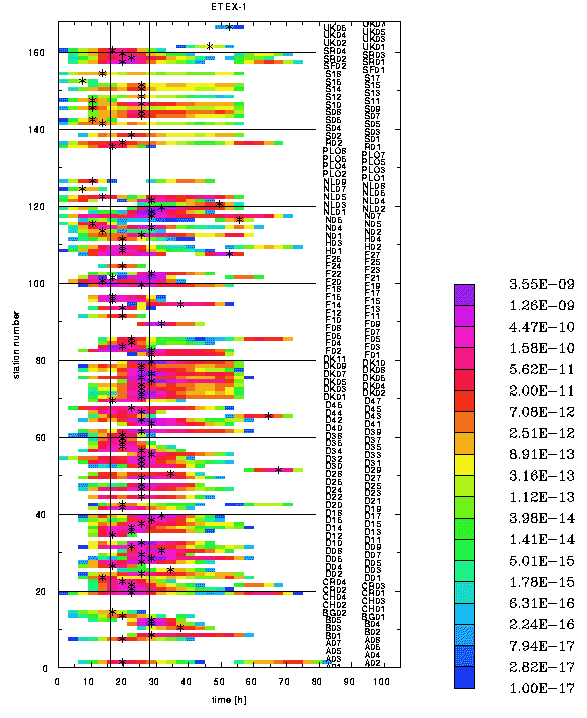
Figure 1: Time series of a tracer* released at the measurements sites
proportional to measured tracer concentrations, sampled at the true
release site. Each line corresponds to one measurement location
(denoted by its ETEX station code) and the sum over all measurement
intervals. Asterisks denote the maxima, and vertical
lines the begin and end of the release. Note the logarithmic
scale.
Figure 1 shows that this method gives already a
good picture of the timing of the release. The maximum lies within
the real release interval for most stations, but some of them
(e.g., D30 = Mannheim in Germany) are clear outliers. Figure 2 gives an
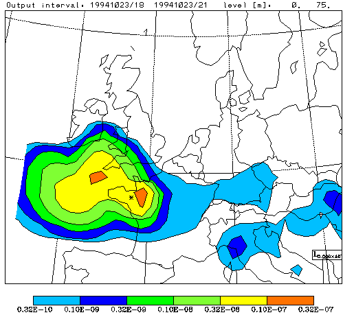
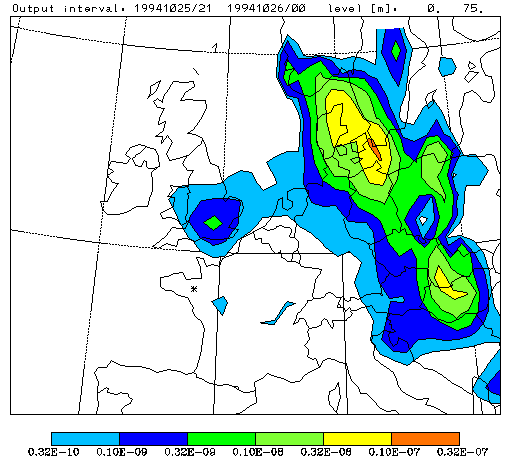
idea how the ``adjoint tracer'' cloud* looks like at different times.
The left frame is at the time of the release and shows its maximum
near the release location while the right frame is at a later time
(previos stage of the backward simulation) and looks similar to the
``real'' cloud at this stage as depicted by measurements. This figure may
be compared with Fig. 3 in [5].


Figure 2: Horizontal distribution of a tracer* released at
the measurements sites proportional to measured tracer concentrations.
Note the logarithmic scale. The real release location is marked by a
hollow black dot. The left (top) panel shows the tracer during the time of the
real release (23 Oct, 18-21 UTC), the right (bottom) panel at a previous stage
of the inverse simulation (25 Oct, 21-24 UTC).
3.4 Inversion of temporal release evolution
We perform a generalised inversion (this means a regularised solution,
see [6]) of the LSE yo » Mx (Eq. 4),
where yo are the observations, minimising the cost function
|
J = || yo - M |
^
x
|
||2 + q2|| |
^
x
|
||2 |
| (8) |
in order to obtain the source x as a function of time, assuming
the location as given. The source-receptor matrix for the release
point is obtained by linear interpolation from the four surrounding
cells. All data are used, and the full time range between 23 Oct
12 UTC and 27 Oct 12 UTC is used, in contrast to [5].
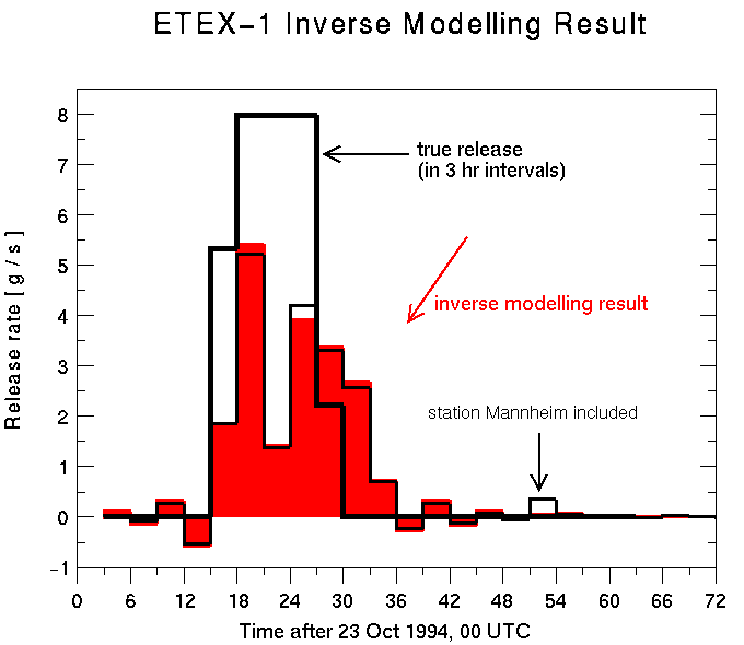
Figure 3 shows the result. We see that the start of the
release was accurately captured. The end of the release was
found well but is too fuzzy and slightly biased towards later times.
As the peak caused by station Mannheim at 50 h shows, the inversion
is disturbed to some extent by outliers.

Figure 3: ETEX Release 1, true time-dependent release rate (merged into
3 h intervals) and release rate obtained by inverse modelling (with and
without the outlier station Mannheim).
Observed concentrations and concentrations computed by
following methods have been compared as a test.
- FWD: Forward simulation made by A. Stohl [8]
with true source term xt
- BWD-i1: Concentrations obtained as M[^(x)] where [^(x)]
denotes the source term estimated by inverse modelling
- BWD-i2: Concentrations obtained as M[^(x)]* where
[^(x)]* = [^(x)] |xt| / |[^(x)]|
(scaled source term)
- BWD-t: Concentrations obtained as M xt (true source term,
transformed to 3 h resolution)
The results are presented in Table 1. We see that the SRM of the
inverse run yields worse results than the forward run, but results with
the reconstructed source term are better than with the real source term
with respect to correlation and RMS error (not, of course, for bias).
The total release is underestimated by 35% inspite of an unbiased
forward simulation. We can thus conclude that the backward simulation
suffers from the 3-hourly temporal and the grid-cell horizontal resolution
of the source. The bias is obviously caused by formulation of cost
function in combination with simulation errors.
Table 1: Statistical performance indicators for the
comparison modelled - measured tracer concentrations. Meaning of
abbreviations for the method see text.
| Method | r | relative bias | relative RMSE | |x|
|
| FWD | 0.59 | » 0.01 | ?(not published) | 340 kg
|
| BWD-i1 | 0.44 | -0.35 | 1.84 | 208 kg
|
| BWD-i2 | 0.44 | +0.05 | 2.99 | 340 kg
|
| BWD-t | 0.33 | +0.13 | 3.51 | 340 kg |
4 Conclusions and outlook
Backward simulations with a LPDM have successfully been
established as a tool for the generation of source-receptor matrices.
This method is attractive with respect to accuracy and
computational effort. It yields useful results already in
this first implementation, and it can be expected that
it will improve after the following steps:
- Test the effect of better temporal resolution of the source.
- Introduce weighting of observations according to the
error associated with them, to reduce the influence of outliers.
- Do inverse modelling for finding the source location and
the joint time-space location.
- Test more sophisticated regularisation methods.
In the future, this method shall be applied also to other tracer
experiments such as ANATEX and CAPTEX as well as to the release from
the Chernobyl NPP disaster. Finally, the method may be used for unknown
sources.
References
- [1]
- Elbern H., and H. Schmidt, A four-dimensional variational chemistry data assimilation scheme for Eulerian
chemistry transport modeling. J. Geophys. Res. 104(D15) (1999), 18,583-18589.
- [2]
- ETEX, a European tracer experiment, Atmos. Environ. 32, Vol. 24 (special issue) (1998).
- [3]
- ETEX. The European tracer experiment, European Communities, Publ. No. EUR 18143EN, ISBN 92-828-5007-2, 107 pp.,
1998.
- [4]
- Pudykiewicz J. A., Application of adjoint tracer transport equations for evaluating source
parameters. Atmos. Environ. 32 (1998), 3039-3050.
- [5]
- Robertson L., and J. Langner, Source function estimate by means of a variational data assimilation applied
to the ETEX-I tracer experiment. Atmos. Environ. 32(24) (1998), 4219-4225.
- [6]
- Seibert P., Inverse modelling of sulfur emissions in Europe based on trajectories, Inverse Methods in Global Biogeochemical Cycles, AGU Geophysical Monograph
Vol. 114, 1999, pp. 147-154.
<
- [7]
- Stohl A., Computation, accuracy and applications of trajectories - a review and bibliography. Atmos. Environ. 32 (1998), 947-966.
- [8]
- Stohl A., M. Hittenberger, G. Wotawa, Validation of the Lagrangian particle dispersion model FLEXPART against
large scale tracer experiments, Atmos. Environ. 32(24) (1998), 4245-4264.
Footnotes:
1 This
work is a contribution to
EUROTRAC-2 subprojects
GLOREAM and
GENEMIS-2, funded by
FWF under P1295-GEO. Meteorological
data from ECMWF have kindly been
provided through ZAMG (Vienna).
2 The following derivation
is restricted to the case without sinks. However, it is intuitively
clear that the LPDM can be applied in the same way also for the linear
case with sinks, as the relative magnitude of any loss along a certain
transport distance is the same in the forward and in the backward
mode. The exact derivation will be presented later.
File translated from TEX by TTH, version 1.94.
On 29 Nov 1999, 17:51.
